scNT-seq human hematopoiesis

In this tutorial, we will show how to estimate dynamics from new/total expressions (labeling) with Model2 from dynamo Cell paper and how our processed hematopoiesis dataset is generated. The corresponding results have been stored in dyn.sample_data.hematopoiesis. We can directly access the processed hematopoiesis dataset based on needs.

In dynamo Cell paper Model2, we take into account labeling (with a labeling correction coefficient) but not splicing. The total RNA has a synthesis rate constant and a degradation rate constant. The labeled RNA has a reduced synthesis rate constant but the same degradation rate constant. For more theoretical parts and ODE equations, please refer to dynamo Cell paper.

%%capture

import dynamo as dyn
import pandas as pd
import numpy as np
import warnings

warnings.filterwarnings("ignore")

Read raw hematopoiesis data via dyn.sample_data.hematopoiesis_raw. new and total layer will be used for dynamics estimation.

adata_hsc_raw = dyn.sample_data.hematopoiesis_raw()
adata_hsc_raw

AnnData object with n_obs × n_vars = 1947 × 26193
    obs: 'batch', 'cell_type', 'time'
    var: 'gene_name_mapping'
    uns: 'genes_to_use'
    obsm: 'X_umap'
    layers: 'new', 'spliced', 'total', 'unspliced'

The following code cells preprocess adata. We use a predefined gene list based on literature review and metrics such as highly variable genes. The gene list is stored in adata_hsc_raw.uns["genes_to_use"] of the hematopoiesis raw dataset we provide

selected_genes_to_use = adata_hsc_raw.uns["genes_to_use"]

dyn.pp.recipe_monocle(
    adata_hsc_raw,
    tkey="time",
    experiment_type="one-shot",
    genes_to_use=selected_genes_to_use,
    n_top_genes=len(selected_genes_to_use),
    # feature_selection_layer="new",
    maintain_n_top_genes=True,
)

|-----> apply Monocole recipe to adata...
|-----> convert ensemble name to official gene name
|-----? Your adata object uses non-official gene names as gene index.
Dynamo is converting those names to official gene names.
[ Future queries will be cached in "/Users/random/dynamo_readthedocs/docs/source/notebooks/mygene_cache.sqlite" ]
querying 1-1000...done. [ from cache ]
querying 1001-2000...done. [ from cache ]
querying 2001-3000...done. [ from cache ]
querying 3001-4000...done. [ from cache ]
querying 4001-5000...done. [ from cache ]
querying 5001-6000...done. [ from cache ]
querying 6001-7000...done. [ from cache ]
querying 7001-8000...done. [ from cache ]
querying 8001-9000...done. [ from cache ]
querying 9001-10000...done. [ from cache ]
querying 10001-11000...done. [ from cache ]
querying 11001-12000...done. [ from cache ]
querying 12001-13000...done. [ from cache ]
querying 13001-14000...done. [ from cache ]
querying 14001-15000...done. [ from cache ]
querying 15001-16000...done. [ from cache ]
querying 16001-17000...done. [ from cache ]
querying 17001-18000...done. [ from cache ]
querying 18001-19000...done. [ from cache ]
querying 19001-20000...done. [ from cache ]
querying 20001-21000...done. [ from cache ]
querying 21001-22000...done. [ from cache ]
querying 22001-23000...done. [ from cache ]
querying 23001-24000...done. [ from cache ]
querying 24001-25000...done. [ from cache ]
querying 25001-26000...done. [ from cache ]
querying 26001-26193...done. [ from cache ]
Finished.
1 input query terms found dup hits:
        [('ENSG00000229425', 2)]
29 input query terms found no hit:
        ['ENSG00000168078', 'ENSG00000189144', 'ENSG00000203812', 'ENSG00000221995', 'ENSG00000225178', 'ENS
Pass "returnall=True" to return complete lists of duplicate or missing query terms.
|-----> <insert> pp to uns in AnnData Object.
|-----------> <insert> has_splicing to uns['pp'] in AnnData Object.
|-----------> <insert> has_labling to uns['pp'] in AnnData Object.
|-----------> <insert> splicing_labeling to uns['pp'] in AnnData Object.
|-----------> <insert> has_protein to uns['pp'] in AnnData Object.
|-----> ensure all cell and variable names unique.
|-----> ensure all data in different layers in csr sparse matrix format.
|-----> ensure all labeling data properly collapased
|-----------> <insert> tkey to uns['pp'] in AnnData Object.
|-----------> <insert> experiment_type to uns['pp'] in AnnData Object.
|-----> filtering cells...
|-----> <insert> pass_basic_filter to obs in AnnData Object.
|-----> 1947 cells passed basic filters.
|-----> filtering gene...
|-----> <insert> pass_basic_filter to var in AnnData Object.
|-----> 2885 genes passed basic filters.
|-----> calculating size factor...
|-----> <insert> use_for_pca to var in AnnData Object.
|-----> <insert> frac to var in AnnData Object.
|-----> size factor normalizing the data, followed by log1p transformation.
|-----> applying PCA ...
|-----> <insert> pca_fit to uns in AnnData Object.
|-----> <insert> ntr to obs in AnnData Object.
|-----> <insert> ntr to var in AnnData Object.
|-----> cell cycle scoring...
|-----> <insert> cell_cycle_phase to obs in AnnData Object.
|-----> <insert> cell_cycle_scores to obsm in AnnData Object.
|-----> [Cell Cycle Scores Estimation] in progress: 100.0000%
|-----> [Cell Cycle Scores Estimation] finished [0.1040s]
|-----> [recipe_monocle preprocess] in progress: 100.0000%
|-----> [recipe_monocle preprocess] finished [2.3393s]

adata_hsc_raw.var.use_for_pca.sum()

1766

dyn.tl.reduceDimension(adata_hsc_raw)

|-----> retrive data for non-linear dimension reduction...
|-----? adata already have basis umap. dimension reduction umap will be skipped!
set enforce=True to re-performing dimension reduction.
|-----> Start computing neighbor graph...
|-----------> X_data is None, fetching or recomputing...
|-----> fetching X data from layer:None, basis:pca
|-----> method arg is None, choosing methods automatically...
|-----------> method ball_tree selected
|-----> <insert> connectivities to obsp in AnnData Object.
|-----> <insert> distances to obsp in AnnData Object.
|-----> <insert> neighbors to uns in AnnData Object.
|-----> <insert> neighbors.indices to uns in AnnData Object.
|-----> <insert> neighbors.params to uns in AnnData Object.
|-----> [dimension_reduction projection] in progress: 100.0000%
|-----> [dimension_reduction projection] finished [0.1038s]

Apply model2 and one-shot modeling

dyn.tl.moments(adata_hsc_raw, group="time")

|-----> calculating first/second moments...

OMP: Info #273: omp_set_nested routine deprecated, please use omp_set_max_active_levels instead.

|-----> [moments calculation] in progress: 100.0000%
|-----> [moments calculation] finished [13.3928s]

Because we have unsplicing/splicing expressions in adata, our preprocess module recognizes it and assumes adata has splicing and labeling. We need to set has_splicing to be false in order to use Model2, which estimates dynamics without unsplicing/splicing and only considers labeling data (new/total).

adata_hsc_raw.uns["pp"]["has_splicing"] = False
dyn.tl.dynamics(adata_hsc_raw, group="time", one_shot_method="sci_fate", model="deterministic");

|-----> calculating first/second moments...
|-----> [moments calculation] in progress: 100.0000%
|-----> [moments calculation] finished [3.3029s]

estimating gamma: 100%|██████████| 1766/1766 [00:08<00:00, 198.98it/s]
estimating alpha: 100%|██████████| 1766/1766 [00:00<00:00, 62856.01it/s]

|-----> calculating first/second moments...
|-----> [moments calculation] in progress: 100.0000%
|-----> [moments calculation] finished [2.2067s]

estimating gamma: 100%|██████████| 1766/1766 [00:06<00:00, 290.13it/s]
estimating alpha: 100%|██████████| 1766/1766 [00:00<00:00, 69459.31it/s]

dyn.tl.cell_velocities(
    adata_hsc_raw,
    enforce=True,
    method="cosine",
);

One-shot labeling modeling

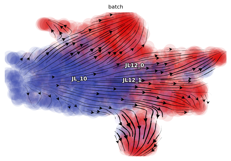
The one-shot labeling model from dynamo was used to estimate absolute total RNA velocities on the labeling data (new and total RNA). Because we quantified both the labeling and splicing information, we used the second formula that involves both splicing and labeling data to define total RNA velocity. The high-dimensional velocity vectors were projected to two- dimensional UMAP space and visualized with the streamline plot, using dynamo with default parameters (Figure 3B). Similarly, the total RNA velocity plot in Figure 3D and total RNA phase diagram in Figure 3E for example gene PF4 were generated using dynamo with default settings.

adata_hsc_raw.obs.time.unique()

array([3, 5])

We have two time points in hsc dataset. Here we split the dataset based on time points and prepare data for calculation next.

pca_genes = adata_hsc_raw.var.use_for_pca
new_expr = adata_hsc_raw[:, pca_genes].layers["M_n"]
gamma = adata_hsc_raw[:, pca_genes].var.gamma
time_3_gamma = adata_hsc_raw[:, pca_genes].var.time_3_gamma.astype(float)
time_5_gamma = adata_hsc_raw[:, pca_genes].var.time_5_gamma.astype(float)

t = adata_hsc_raw.obs.time.astype(float)
M_s = adata_hsc_raw.layers["M_s"][:, pca_genes]

time_3_cells = adata_hsc_raw.obs.time == 3
time_5_cells = adata_hsc_raw.obs.time == 5

Next, we will calculate velocity_alpha_minus_gamma_s according to

\[\alpha = new / (1 - e^{-rt}) \cdot r\]

def alpha_minus_gamma_s(new, gamma, t, M_s):
    # equation: alpha = new / (1 - e^{-rt}) * r
    alpha = new.A.T / (1 - np.exp(-gamma.values[:, None] * t.values[None, :])) * gamma.values[:, None]

    gamma_s = gamma.values[:, None] * M_s.A.T
    alpha_minus_gamma_s = alpha - gamma_s
    return alpha_minus_gamma_s

time_3_velocity_n = alpha_minus_gamma_s(new_expr[time_3_cells, :], time_3_gamma, t[time_3_cells], M_s[time_3_cells, :])
time_5_velocity_n = alpha_minus_gamma_s(new_expr[time_5_cells, :], time_5_gamma, t[time_5_cells], M_s[time_5_cells, :])

velocity_n = adata_hsc_raw.layers["velocity_N"].copy()

valid_velocity_n = velocity_n[:, pca_genes].copy()
valid_velocity_n[time_3_cells, :] = time_3_velocity_n.T
valid_velocity_n[time_5_cells, :] = time_5_velocity_n.T
velocity_n[:, pca_genes] = valid_velocity_n.copy()

adata_hsc_raw.layers["velocity_alpha_minus_gamma_s"] = velocity_n.copy()

The results are stored in adata_hsc_raw.layers["velocity_alpha_minus_gamma_s"], which can be further projected to low dimension space for visualization.

dyn.tl.cell_velocities(
    adata_hsc_raw,
    enforce=True,
    X=adata_hsc_raw.layers["M_t"],
    V=adata_hsc_raw.layers["velocity_alpha_minus_gamma_s"],
    method="cosine",
);
dyn.pl.streamline_plot(
    adata_hsc_raw,
    color=["batch"],
    ncols=4,
    basis="umap",
)