scEU-seq cell cycle

This tutorial uses the cell cycle dataset from Battich, et al (2020). This tutorial is the first one of the two tutorials for demonstrating how dynamo can use used to analyze the scEU-seq data. Please refer the organoid tutorial for details on how to analyze the organoid dataset.

Recently Battich and colleague reported scEU-seq as a method to sequence mRNA labeled with 5-ethynyl-uridine (EU) in single cells. By developing a very creative labeling strategy (personally this is my favorite labeling strategy from all available labeling based scRNA-seq papers!) they are able to estimate of RNA transcription and degradation rates in single cell across time.

They applied scEU-seq and the labeling strategy to study the transcription and degradation rates for both the cell cycle eand differentiation processes. Similar to what has been discovered in bulk studies, they find the transcription rates are highly dynamic while the degration rate tend to be more stable across different time points. Furthermore, by quantifying the correlation between the transcription rate and degration rates across time, they reveal major regulatory strategies which have distinct consequences for controlling the dynamic range and precision of gene expression.

For both of the cell cycle and the organoid systems, the authors use kinetics and a mixture of pulse and chase experiment to label the cells. I had a lot fun to analyze this complicate dataset. But for the sake of simplicity, here I am going to only use the fraction of kinetics experiment for demonstrating how dynamo can be used to estimate labeling based RNA velocity and to reconstruct vector field function.

# get the latest pypi version
# to get the latest version on github and other installations approaches, see:
# https://dynamo-release.readthedocs.io/en/latest/ten_minutes_to_dynamo.html#how-to-install
!pip install dynamo-release --upgrade --quiet

import warnings
warnings.filterwarnings('ignore')

import dynamo as dyn
import anndata
import pandas as pd
import numpy as np
import scipy.sparse

from anndata import AnnData
from scipy.sparse import csr_matrix

dyn.get_all_dependencies_version()

package	dynamo-release	umap-learn	anndata	cvxopt	hdbscan	loompy	matplotlib	numba	numpy	pandas	pynndescent	python-igraph	scikit-learn	scipy	seaborn	setuptools	statsmodels	tqdm	trimap	numdifftools	colorcet
version	0.95.2	0.4.6	0.7.4	1.2.3	0.8.26	3.0.6	3.3.0	0.51.0	1.19.1	1.1.1	0.4.8	0.8.2	0.23.2	1.5.2	0.9.0	49.6.0	0.11.1	4.48.2	1.0.12	0.9.39	2.0.2

Load data

Let us first take a look at number of cells collected at time labeling time point for either the pulse or chase experiment.

rpe1 = dyn.read('/Users/xqiu/Dropbox (Personal)/dynamo/dont_remove/rpe1.h5ad')

rpe1

AnnData object with n_obs × n_vars = 5422 × 11848
    obs: 'Plate_Id', 'Condition_Id', 'Well_Id', 'RFP_log10_corrected', 'GFP_log10_corrected', 'Cell_cycle_possition', 'Cell_cycle_relativePos', 'exp_type', 'time'
    var: 'Gene_Id'
    layers: 'sl', 'su', 'ul', 'uu'

rpe1.obs.exp_type.value_counts()

Pulse    3058
Chase    2364
Name: exp_type, dtype: int64

rpe1[rpe1.obs.exp_type=='Chase', :].obs.time.value_counts()

   541
     460
    436
   391
   334
dmso    202
Name: time, dtype: int64

rpe1[rpe1.obs.exp_type=='Pulse', :].obs.time.value_counts()

    574
    564
    442
   408
    405
   400
dmso    265
Name: time, dtype: int64

Subset the kinetics experimetn data

For the sake of simplicity, I am going to just focus on the kinetics experiment dataset analysis.

rpe1_kinetics = rpe1[rpe1.obs.exp_type=='Pulse', :]
rpe1_kinetics.obs['time'] = rpe1_kinetics.obs['time'].astype(str)
rpe1_kinetics.obs.loc[rpe1_kinetics.obs['time'] == 'dmso', 'time'] = -1
rpe1_kinetics.obs['time'] = rpe1_kinetics.obs['time'].astype(float)
rpe1_kinetics = rpe1_kinetics[rpe1_kinetics.obs.time != -1, :]

rpe1_kinetics.layers['new'], rpe1_kinetics.layers['total'] = rpe1_kinetics.layers['ul'] + rpe1_kinetics.layers['sl'], rpe1_kinetics.layers['su'] + rpe1_kinetics.layers['sl'] + rpe1_kinetics.layers['uu'] + rpe1_kinetics.layers['ul']

del rpe1_kinetics.layers['uu'], rpe1_kinetics.layers['ul'], rpe1_kinetics.layers['su'], rpe1_kinetics.layers['sl']

Trying to set attribute .obs of view, copying.

rpe1_kinetics

AnnData object with n_obs × n_vars = 2793 × 11848
    obs: 'Plate_Id', 'Condition_Id', 'Well_Id', 'RFP_log10_corrected', 'GFP_log10_corrected', 'Cell_cycle_possition', 'Cell_cycle_relativePos', 'exp_type', 'time'
    var: 'Gene_Id'
    layers: 'new', 'total'

Perform a typical dynamo analysis

A typical analysis in dynamo includes:

the preprocessing procedure;
kinetic estimation and velocity calculation;
dimension reduction;
high dimension velocity projection;
vector field reconstruction

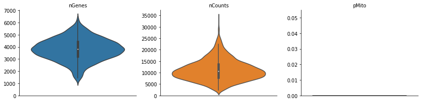
Note that in the preprocess stages, we calculate some basic statistics, the number of genes, total UMI counts and percentage of mitochondrian UMIs in each cell so we can visualize them via dyn.pl.basic_stats. Moreover, if the adata.var_name is not official gene names but ensemble gene ids, dynamo will try to automatically convert those gene ids into human readable official gene names.

dyn.pl.basic_stats(rpe1_kinetics)

_images/scEU_seq_rpe1_analysis_kinetic_13_0.png

rpe1_genes = ['UNG', 'PCNA', 'PLK1', 'HPRT1']

rpe1_kinetics.obs.time

Cell_02365     15.0
Cell_02366     30.0
Cell_02367     30.0
Cell_02368     30.0
Cell_02369     45.0
              ...
Cell_05418    120.0
Cell_05419    120.0
Cell_05420    180.0
Cell_05421    180.0
Cell_05422    180.0
Name: time, Length: 2793, dtype: float64

dyn.pp.recipe_monocle(rpe1_kinetics, n_top_genes=1000, total_layers=False)
rpe1_kinetics.obs.time  = rpe1_kinetics.obs.time.astype('float')
rpe1_kinetics.obs.time = rpe1_kinetics.obs.time/60

querying 1-1000...done.
querying 1001-2000...done.
querying 2001-3000...done.
querying 3001-4000...done.
querying 4001-5000...done.
querying 5001-6000...done.
querying 6001-7000...done.
querying 7001-8000...done.
querying 8001-9000...done.
querying 9001-10000...done.
querying 10001-11000...done.
querying 11001-11848...done.
Finished.
1 input query terms found dup hits:
    [('ENSG00000229425', 2)]
29 input query terms found no hit:
    ['ENSG00000116957', 'ENSG00000168078', 'ENSG00000189144', 'ENSG00000205664', 'ENSG00000213846', 'ENS
Pass "returnall=True" to return complete lists of duplicate or missing query terms.

rpe1_kinetics.obs.time.value_counts()

50    574
75    564
25    442
00    408
00    405
00    400
Name: time, dtype: int64

Estimate time-resolved RNA velocity

There are some very non-trivial consideration between estimating time-resolved RNA velocity and estimating transcription/degration kinetics rates. The following code provides the right strategy for time-resolved RNA velocity analysis. Wait for our final publication for more in-depth discussion in this interesting topic!

dyn.tl.dynamics(rpe1_kinetics, model='deterministic', tkey='time', assumption_mRNA='ss')
dyn.tl.reduceDimension(rpe1_kinetics, reduction_method='umap')

estimating gamma: 100%|██████████| 1000/1000 [00:10<00:00, 92.58it/s]

AnnData object with n_obs × n_vars = 2793 × 11819
    obs: 'Plate_Id', 'Condition_Id', 'Well_Id', 'RFP_log10_corrected', 'GFP_log10_corrected', 'Cell_cycle_possition', 'Cell_cycle_relativePos', 'exp_type', 'time', 'nGenes', 'nCounts', 'pMito', 'use_for_pca', 'Size_Factor', 'initial_cell_size', 'total_Size_Factor', 'initial_total_cell_size', 'new_Size_Factor', 'initial_new_cell_size', 'ntr', 'cell_cycle_phase'
    var: 'Gene_Id', 'query', 'scopes', '_id', '_score', 'symbol', 'notfound', 'pass_basic_filter', 'score', 'log_cv', 'log_m', 'use_for_pca', 'ntr', 'beta', 'gamma', 'half_life', 'alpha_b', 'alpha_r2', 'gamma_b', 'gamma_r2', 'gamma_logLL', 'delta_b', 'delta_r2', 'uu0', 'ul0', 'su0', 'sl0', 'U0', 'S0', 'total0', 'use_for_dynamics'
    uns: 'velocyto_SVR', 'pp_norm_method', 'PCs', 'explained_variance_ratio_', 'pca_fit', 'feature_selection', 'dynamics', 'neighbors', 'umap_fit'
    obsm: 'X_pca', 'X', 'cell_cycle_scores', 'X_umap'
    layers: 'new', 'total', 'X_total', 'X_new', 'M_t', 'M_tt', 'M_n', 'M_tn', 'M_nn', 'velocity_T'
    obsp: 'moments_con', 'connectivities', 'distances'

rpe1_kinetics

AnnData object with n_obs × n_vars = 2793 × 11819
    obs: 'Plate_Id', 'Condition_Id', 'Well_Id', 'RFP_log10_corrected', 'GFP_log10_corrected', 'Cell_cycle_possition', 'Cell_cycle_relativePos', 'exp_type', 'time', 'nGenes', 'nCounts', 'pMito', 'use_for_pca', 'Size_Factor', 'initial_cell_size', 'total_Size_Factor', 'initial_total_cell_size', 'new_Size_Factor', 'initial_new_cell_size', 'ntr', 'cell_cycle_phase'
    var: 'Gene_Id', 'query', 'scopes', '_id', '_score', 'symbol', 'notfound', 'pass_basic_filter', 'score', 'log_cv', 'log_m', 'use_for_pca', 'ntr', 'beta', 'gamma', 'half_life', 'alpha_b', 'alpha_r2', 'gamma_b', 'gamma_r2', 'gamma_logLL', 'delta_b', 'delta_r2', 'uu0', 'ul0', 'su0', 'sl0', 'U0', 'S0', 'total0', 'use_for_dynamics'
    uns: 'velocyto_SVR', 'pp_norm_method', 'PCs', 'explained_variance_ratio_', 'pca_fit', 'feature_selection', 'dynamics', 'neighbors', 'umap_fit'
    obsm: 'X_pca', 'X', 'cell_cycle_scores', 'X_umap'
    layers: 'new', 'total', 'X_total', 'X_new', 'M_t', 'M_tt', 'M_n', 'M_tn', 'M_nn', 'velocity_T'
    obsp: 'moments_con', 'connectivities', 'distances'

dyn.tl.cell_velocities(rpe1_kinetics, enforce=True, vkey='velocity_T', ekey='M_t')

calculating transition matrix via pearson kernel with sqrt transform.: 100%|██████████| 2793/2793 [00:06<00:00, 457.19it/s]
projecting velocity vector to low dimensional embedding...: 100%|██████████| 2793/2793 [00:00<00:00, 4051.10it/s]

AnnData object with n_obs × n_vars = 2793 × 11819
    obs: 'Plate_Id', 'Condition_Id', 'Well_Id', 'RFP_log10_corrected', 'GFP_log10_corrected', 'Cell_cycle_possition', 'Cell_cycle_relativePos', 'exp_type', 'time', 'nGenes', 'nCounts', 'pMito', 'use_for_pca', 'Size_Factor', 'initial_cell_size', 'total_Size_Factor', 'initial_total_cell_size', 'new_Size_Factor', 'initial_new_cell_size', 'ntr', 'cell_cycle_phase'
    var: 'Gene_Id', 'query', 'scopes', '_id', '_score', 'symbol', 'notfound', 'pass_basic_filter', 'score', 'log_cv', 'log_m', 'use_for_pca', 'ntr', 'beta', 'gamma', 'half_life', 'alpha_b', 'alpha_r2', 'gamma_b', 'gamma_r2', 'gamma_logLL', 'delta_b', 'delta_r2', 'uu0', 'ul0', 'su0', 'sl0', 'U0', 'S0', 'total0', 'use_for_dynamics', 'use_for_transition'
    uns: 'velocyto_SVR', 'pp_norm_method', 'PCs', 'explained_variance_ratio_', 'pca_fit', 'feature_selection', 'dynamics', 'neighbors', 'umap_fit', 'grid_velocity_umap'
    obsm: 'X_pca', 'X', 'cell_cycle_scores', 'X_umap', 'velocity_umap'
    layers: 'new', 'total', 'X_total', 'X_new', 'M_t', 'M_tt', 'M_n', 'M_tn', 'M_nn', 'velocity_T'
    obsp: 'moments_con', 'connectivities', 'distances', 'pearson_transition_matrix'

rpe1_kinetics.obsm['X_RFP_GFP'] = rpe1_kinetics.obs.loc[:, ['RFP_log10_corrected', 'GFP_log10_corrected']].values.astype('float')
rpe1_kinetics.layers['velocity_S'] = rpe1_kinetics.layers['velocity_T'].copy()
dyn.tl.cell_velocities(rpe1_kinetics, enforce=True, vkey='velocity_S', ekey='M_t', basis='RFP_GFP')

rpe1_kinetics.obs.Cell_cycle_relativePos = rpe1_kinetics.obs.Cell_cycle_relativePos.astype(float)
rpe1_kinetics.obs.Cell_cycle_possition = rpe1_kinetics.obs.Cell_cycle_possition.astype(float)

calculating transition matrix via pearson kernel with sqrt transform.: 100%|██████████| 2793/2793 [00:06<00:00, 415.17it/s]
projecting velocity vector to low dimensional embedding...: 100%|██████████| 2793/2793 [00:00<00:00, 3591.64it/s]

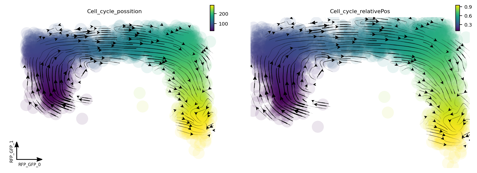
Visualize velocity streamlines

When we project our estimated transcriptomic RNA velocity to the space formed by the \(log_{10}(fluorescence), Geminin -GFP\) and \(log_{10}(fluorescence), Cdt1-RFP\) (Geminin and Cdt1 are two markers of different cell cycle stages), we can a nice transition from early cell cycle stage to late cell cycle stage.

dyn.pl.streamline_plot(rpe1_kinetics, color=['Cell_cycle_possition', 'Cell_cycle_relativePos'], basis='RFP_GFP')

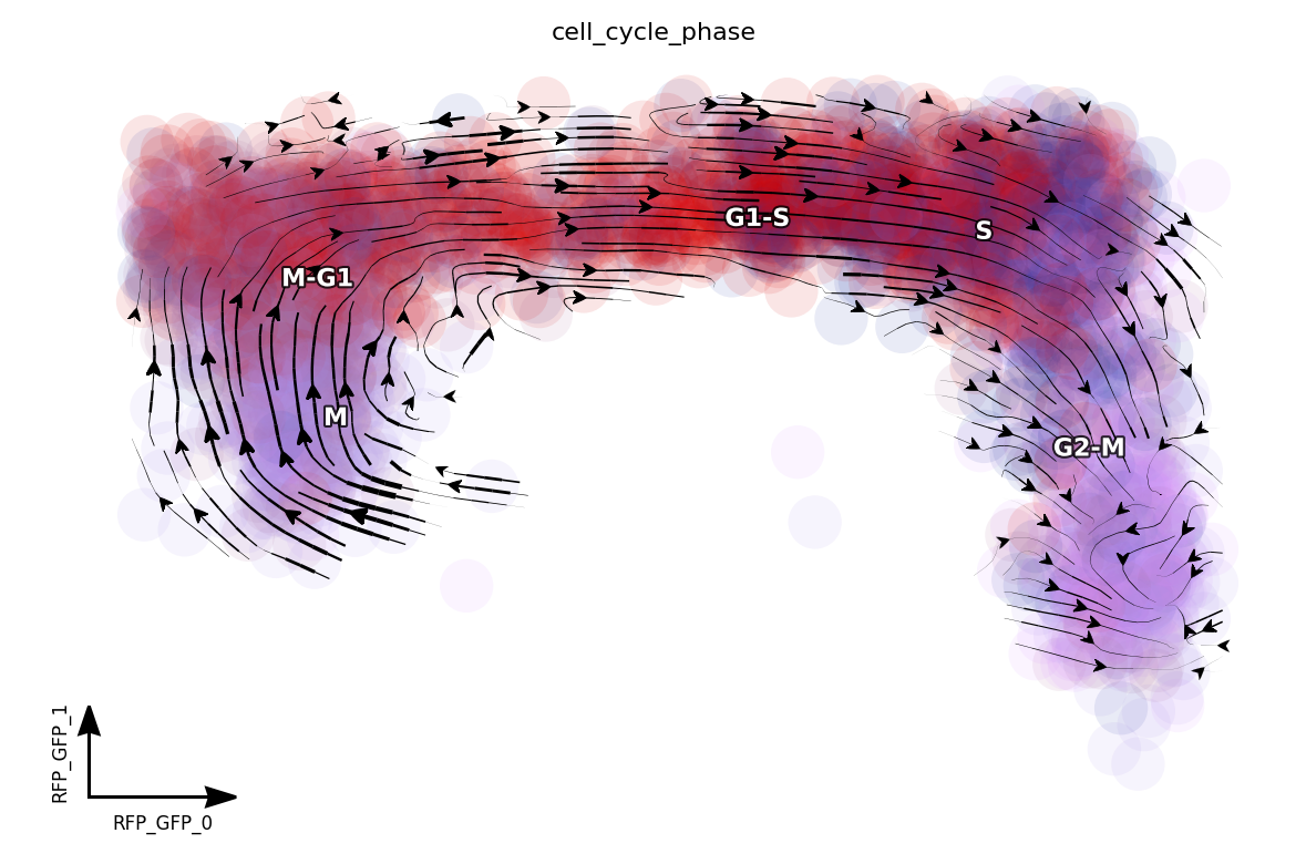
_images/scEU_seq_rpe1_analysis_kinetic_24_0.png

Since dynamo automatically performs the cell cycle staging at the preprocess step with cell-cycle related marker genes using methods from Norman et. al. We can also check whether dynamo’s staging makes any sense for this dataset. Interesting, dynamo staging indeed reveals a nice transition from M stage to M-G, to G1-S, to S and finally to G2-M stage. This is awesome!

dyn.pl.streamline_plot(rpe1_kinetics, color=['cell_cycle_phase'], basis='RFP_GFP')

<Figure size 600x400 with 0 Axes>

_images/scEU_seq_rpe1_analysis_kinetic_26_1.png

Animate cell cycle transition

dyn.vf.VectorField(rpe1_kinetics, basis='RFP_GFP')

AnnData object with n_obs × n_vars = 2793 × 11819
    obs: 'Plate_Id', 'Condition_Id', 'Well_Id', 'RFP_log10_corrected', 'GFP_log10_corrected', 'Cell_cycle_possition', 'Cell_cycle_relativePos', 'exp_type', 'time', 'nGenes', 'nCounts', 'pMito', 'use_for_pca', 'Size_Factor', 'initial_cell_size', 'total_Size_Factor', 'initial_total_cell_size', 'new_Size_Factor', 'initial_new_cell_size', 'ntr', 'cell_cycle_phase'
    var: 'Gene_Id', 'query', 'scopes', '_id', '_score', 'symbol', 'notfound', 'pass_basic_filter', 'score', 'log_cv', 'log_m', 'use_for_pca', 'ntr', 'beta', 'gamma', 'half_life', 'alpha_b', 'alpha_r2', 'gamma_b', 'gamma_r2', 'gamma_logLL', 'delta_b', 'delta_r2', 'uu0', 'ul0', 'su0', 'sl0', 'U0', 'S0', 'total0', 'use_for_dynamics', 'use_for_transition'
    uns: 'velocyto_SVR', 'pp_norm_method', 'PCs', 'explained_variance_ratio_', 'pca_fit', 'feature_selection', 'dynamics', 'neighbors', 'umap_fit', 'grid_velocity_umap', 'grid_velocity_RFP_GFP', 'VecFld_RFP_GFP', 'VecFld'
    obsm: 'X_pca', 'X', 'cell_cycle_scores', 'X_umap', 'velocity_umap', 'X_RFP_GFP', 'velocity_RFP_GFP', 'velocity_RFP_GFP_SparseVFC', 'X_RFP_GFP_SparseVFC'
    layers: 'new', 'total', 'X_total', 'X_new', 'M_t', 'M_tt', 'M_n', 'M_tn', 'M_nn', 'velocity_T', 'velocity_S'
    obsp: 'moments_con', 'connectivities', 'distances', 'pearson_transition_matrix'

progenitor = rpe1_kinetics.obs_names[rpe1_kinetics.obs.Cell_cycle_relativePos < 0.1]
len(progenitor)

np.random.seed(19491001)

from matplotlib import animation
info_genes = rpe1_kinetics.var_names[rpe1_kinetics.var.use_for_transition]
dyn.pd.fate(rpe1_kinetics, basis='RFP_GFP', init_cells=progenitor, interpolation_num=100,  direction='forward',
   inverse_transform=False, average=False)

integration with ivp solver: 100%|██████████| 78/78 [00:10<00:00,  7.15it/s]
uniformly sampling points along a trajectory: 100%|██████████| 78/78 [00:00<00:00, 287.20it/s]

AnnData object with n_obs × n_vars = 2793 × 11819
    obs: 'Plate_Id', 'Condition_Id', 'Well_Id', 'RFP_log10_corrected', 'GFP_log10_corrected', 'Cell_cycle_possition', 'Cell_cycle_relativePos', 'exp_type', 'time', 'nGenes', 'nCounts', 'pMito', 'use_for_pca', 'Size_Factor', 'initial_cell_size', 'total_Size_Factor', 'initial_total_cell_size', 'new_Size_Factor', 'initial_new_cell_size', 'ntr', 'cell_cycle_phase'
    var: 'Gene_Id', 'query', 'scopes', '_id', '_score', 'symbol', 'notfound', 'pass_basic_filter', 'score', 'log_cv', 'log_m', 'use_for_pca', 'ntr', 'beta', 'gamma', 'half_life', 'alpha_b', 'alpha_r2', 'gamma_b', 'gamma_r2', 'gamma_logLL', 'delta_b', 'delta_r2', 'uu0', 'ul0', 'su0', 'sl0', 'U0', 'S0', 'total0', 'use_for_dynamics', 'use_for_transition'
    uns: 'velocyto_SVR', 'pp_norm_method', 'PCs', 'explained_variance_ratio_', 'pca_fit', 'feature_selection', 'dynamics', 'neighbors', 'umap_fit', 'grid_velocity_umap', 'grid_velocity_RFP_GFP', 'VecFld_RFP_GFP', 'VecFld', 'fate_RFP_GFP'
    obsm: 'X_pca', 'X', 'cell_cycle_scores', 'X_umap', 'velocity_umap', 'X_RFP_GFP', 'velocity_RFP_GFP', 'velocity_RFP_GFP_SparseVFC', 'X_RFP_GFP_SparseVFC'
    layers: 'new', 'total', 'X_total', 'X_new', 'M_t', 'M_tt', 'M_n', 'M_tn', 'M_nn', 'velocity_T', 'velocity_S'
    obsp: 'moments_con', 'connectivities', 'distances', 'pearson_transition_matrix'

%%capture
import matplotlib.pyplot as plt

fig, ax = plt.subplots()
ax = dyn.pl.topography(rpe1_kinetics, basis='RFP_GFP', color='Cell_cycle_relativePos', ax=ax, save_show_or_return='return')
ax.set_aspect(0.8)

%%capture
instance = dyn.mv.StreamFuncAnim(adata=rpe1_kinetics, basis='RFP_GFP', color='Cell_cycle_relativePos', ax=ax)

import matplotlib
matplotlib.rcParams['animation.embed_limit'] = 2**128 # Ensure all frames will be embedded.

from matplotlib import animation
import numpy as np

anim = animation.FuncAnimation(instance.fig, instance.update, init_func=instance.init_background,
                               frames=np.arange(100), interval=100, blit=True)
from IPython.core.display import display, HTML
HTML(anim.to_jshtml()) # embedding to jupyter notebook.